Principle Foundations Home Page
![]()
Problems in Regression Analysis
and
their Corrections
![]()
Multicollinearity
refers to the case in which two or more explanatory variables in the
regression model are highly correlated, making it difficult or impossible
to isolate their individual effects on the dependent variable. With
multicollinearity, the estimated OLS coefficients may be statistically
insignificant (and even have the wrong sign) even though R2 may
be "high". Multicollinearity can some times be overcome or
reduced by collecting more data, by utilizing a priory information, by
transforming the functional relationship, or by dropping one of the higly
collinear variables.
Two
or more independent variables are perfectly collinear if one or more of
the variables can be expressed as a linear combination of the other
variable(s). For example, there is perfect multicollinearity between X1
and X2 if X1 = 2X2 or
![]() . If two or more explanatory variables are perfectly linearly correlated,
it will be impossible to calculate OLS estimates of the parameters because
the system of normal equations will contain two or more equations that are
not independent.
. If two or more explanatory variables are perfectly linearly correlated,
it will be impossible to calculate OLS estimates of the parameters because
the system of normal equations will contain two or more equations that are
not independent.
High,
but not perfect, multicollinearity refers to the case in which two or more
independent variables in the regression model are highly correlated. This
may make it difficult or impossible to isolate the effect that each of the
highly collinear explanatory variables has on the dependent variable.
However, The OLS estimated coefficients are still unbiased (if the model
is properly specified). Furthermore, if the principal aim is prediction,
multicollinearity is not a problem if the same multicollinearity pattern
persists during the forecasted period.
The
classic case of multicollinearity occurs when none of explanatory
variables in the OLS regression is statistically significant (an some may
even have the wrong sign), even though R2 may be high (say,
between 0.7 and 1.0). In the less clear-cut cases, detecting
multicollinearity may be more difficult. High, simple, or partial
correlation coefficients amongst explanatory variables are sometimes used
as a measure of multicollinearity. However, serious multicollinearity can
be present even if simple or partial correlation coefficients are
relatively low (ie less than 0.5).
Serious
multicollinearity may sometimes be corrected by 1) extending the size of the sample data,
2) utilizing a priory information (for example, we may know from a previous
study that b2=0.25b1), 3) transforming the functional
relationship, or 4) dropping one of the highly collinear variables
(however, this may lead to specification bias or error if theory tells us
that the dropped variable should be included in the model).
If
the OLS assumption that the variance of the error term is constant for all
values of the independent variables does not hold, we face the problem of
heteroskedasticity. This leads to unbiased but inefficient (ie, larger
than minimum variance) estimates of the standard errors (and thus,
incorrect statistical tests confidence intervals).
One test for heteroskedasticity involves arranging the data from small to large values of the independent variable, X, and running two regressions, one for small values of X and one for large values, omitting, say, one-fifth of the middle observations. Then, we test that the ratio of the error sum of squares (ESS) of the second to the first regression is significantly different from zero, using the F table with (n-d-2k)/2 d.f, where n is the total number of observations, d is the numbers of omitted observations and K is the number of estimated parameters.
If
the error variance is proportional to X2 (often the case),
heteroskedasticity can be overcome by dividing every term of the model by
X and then reestimating the regression using the transformed variables.
Heteroskedasticity
refers to the case in which the variance of the error term is not constant
for all values of the independent variable. That is,
![]() , so
, so
![]() . This violates the third assumption of the OLS regression model. it
occurs primarily in cross sectional data. For example, the error variance
associated with the expenditures of low-income families is usually smaller
than for high-income families because most of the expenditures of
low-income families are on necessities, with little room for discretion.
. This violates the third assumption of the OLS regression model. it
occurs primarily in cross sectional data. For example, the error variance
associated with the expenditures of low-income families is usually smaller
than for high-income families because most of the expenditures of
low-income families are on necessities, with little room for discretion.
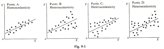
Figure
9-1a shows homoskedastic (i.e., constant variance) disturbances, while
Figure 9-1b, c, and d shows heteroskedastic disturbances. In Figure 9-1b,
![]() increases with Xi.
In Figure 9-1c,
increases with Xi.
In Figure 9-1c,
![]() decreases with Χi.
In Figure 9-1d,
decreases with Χi.
In Figure 9-1d,
![]() first decreases and then
increases as Xi increases. In economics, the heteroskedasticity
shown in Figure 9-1b is the most common, so the discussion that follows
refers to that.
first decreases and then
increases as Xi increases. In economics, the heteroskedasticity
shown in Figure 9-1b is the most common, so the discussion that follows
refers to that.
With
heteroskedasticity, the OLS parameter estimate are still unbiased and
consistent, but they are inefficient (i.e., they have larger than minimum
variances). Furthermore, the estimated variances of the parameters are
biased, leading to incorrect statistical tests for the parameters and
biased confidence intervals.
The
presence of heteroskedasticity can be tested by arranging the data from
small to large values of the independent variable, Xi, and then
running two separate regressions, one for small values of Xi
and one for large values of Xi, omitting some (say, one-fifth)
of the middle observations. Then the ratio of the error sum of squares of
the second regression to the error sum of squares of the first regression
(that is, ESS2/ESS1) is tested to see if it is
significantly different from zero. The F distribution is used for this
test with (n - d -2k)/2 degrees of freedom, where n is the total number of
observations, d is the number of omitted observations, and k is the number
of estimated parameters. This is the Goldfeld-Quandt test for heteroskedasticity and is most appropriate for large samples (i.e.,
for
![]() ). If no middle observations are omitted, the test is still correct, but
it will have a reduced power to detect heteroskedasticity.
). If no middle observations are omitted, the test is still correct, but
it will have a reduced power to detect heteroskedasticity.
When
the error term in one time period is positively correlated with the error
term in the previous time period, we face the problem of (positive
first-order) autocorrelation. This is common in time-series analysis and
leads to downward-biased standard errors (and, thus, to incorrect
statistical tests and confidence intervals).
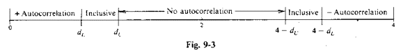
The
presence of first-order auto relation is tested by utilizing the table of
the Durbin-Watson statistic (App.8) at the 5 or 1% levels of significance
for n observations and k' explanatory variables. If the calculated value
of d from Eq.(9.1) is smaller than the tabular value of dL
(lower limit), the hypothesis of positive first-order autocorrelation is
accepted.
the
hypothesis is rejected if d>dU (upper limit), and the test
is inconclusive if dL<d<dU.
Autocorrelation
or serial-correlation refers to the case in which the error term in one
time period is correlated with the error term in any other time period. If
the error term in one time period is correlated with the error term in the
previous time period, there is first-order autocorrelation. Most of the
applications in econometrics involve first rather than second- or
higher-order autocorrelation. Most of the applications in econ0ometrics
involve first rather than second-or higher-order autocorrelation. Even
though negative autocorrelation is negative is possible, most economic
time series exhibit positive autocorrelation. Positive, first-order serial
or autocorrelation means that
![]() , thus violating the fourth OLS assumption. This is common in time-series
analysis.
, thus violating the fourth OLS assumption. This is common in time-series
analysis.
Figure
9-2a shows positive and Figure 9-2b shows negative first-order
autocorrelation. Whenever several consecutive residuals have the same sign
as in Figure 9-2a, there is positive first-order autocorrelation. However,
whenever consecutive residuals change sign frequently, as in Figure 9-2b,
there is negative first-order autocorrelation.

With
autocorrelation, the OLS parameter estimates are still unbiased and
consistent, but the standard errors of the estimated regression parameters
are biased, leading to incorrect statistical tests and biased confidence
intervals. With positive first-order autocorrelation, the standard errors
of the estimated regression parameters are biased downward, thus
exaggerating the precision and statistical significance of the estimated
regression parameters.
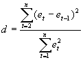
The
presence of autocorrelation can be tested by calculating the Durbin-Watson
statistic, d, given by Eq.(9.1). This is routinely given by most computer
programs such as SPSS:

The
calculated value of d ranges between 0 and 4, with no autocorrelation when
d is in the neighborhood of 2. The values of d indicating the presence or
absence of positive or negative first-order autocorrelation, and for which
the test is inconclusive, are summarized in Figure 9-3. When the lagged
dependent appears as an explanatory variable in the regression, d is
biased toward 2 and its power to detect autocorrelation is hampered.
One
method to correct positive first-order autocorrelation (the usual type)
involves first regressing Y on its value lagged one period, the
explanatory variable of the model, and the explanatory variable lagged one
period:
Yt
= b0(1-p) + pYt-1 + b1Xt -b1pXt
- 1 + ut
(9.2)
(the
preceding equation is derived by multiplying each term of the original OLS
model lagged one period by p, subtracting the resulting expression from
the original OLS model, transposing the term pYt-1 from the left to the
right side of the equation, and defining
ut =ut -put-1). The second step
involves using the value of p founding Eq.(9.2) to transform all the
variables of the original OLS model, as indicated in Eq.(9.3), and
then estimating Eq.(9.3):
![]() (9.3)
(9.3)
The
new error term, ut, in Eq.(9.3) is now free of autocorrelation.
This procedure is known as the Durbin two-stage method and is an example
of generalized least squares. To avoid losing the first observation in the
differencing process,
![]() and
and
![]() is used for the first transformed observation of Y and X, respectively. If
the autocorrelation is due to the omission of an important variable, wrong
functional form, or improper model specification, these problems should be
removed first, before applying the preceding correction procedure for
autocorrelation.
is used for the first transformed observation of Y and X, respectively. If
the autocorrelation is due to the omission of an important variable, wrong
functional form, or improper model specification, these problems should be
removed first, before applying the preceding correction procedure for
autocorrelation.
ERRORS
IN VARIABLES
Errors
in variables refer to the case in which the variables in the regression
model include measurement errors. Measurement errors in the dependent
variable are incorporated into the disturbance term and do not create any
special problem. However, errors in the explanatory variables lead to
biased and inconsistent parameter estimates.
One
method of obtaining consistent OLS parameter estimates is to replace the
explanatory variable subject to measurement errors with another variable
(called an instrumental variable) that is highly correlated with the
original explanatory variable but is independent of the error term. This
is often difficult to do and somewhat arbitrary. The simplest instrument
variable is usually the lagged explanatory variable in question. Another
method used when only X is subject to measurement errors involves
regressing X on Y.
Errors
in variables refer to the case in which the variables in the regression
model include measurement errors. These are probably very common in view
of the way most data are collected and elaborated.![]() is biased downward,
is biased downward,
![]() is biased upward.
is biased upward.
There
is no formal test to detect the presence of errors in variables. Only
economic theory and knowledge of hoe the data were gathered can sometimes
give some indication of the seriousness of the problem.
One
method of obtaining consistent (but still biased and inefficient) OLS
parameter estimates is to replace the explanatory variable subject to
measurement errors with another variable that is highly correlated with an
explanatory variable in question but which is independent of the error
term. In the real world, it might be difficult to find such an
instrumental variable and one could never be sure that it would be
independent of the error term. The most popular instrumental variable is
the lagged value of the explanatory variable in question. Measurement
errors in the explanatory variable also can be corrected by inverse least
squares. This involves regressing X on Y. Then
![]() and
and
![]() , where
, where
![]() and
and
![]() are consistent estimates of the intercept and slope parameter of the
regression of Yt on Xt.
are consistent estimates of the intercept and slope parameter of the
regression of Yt on Xt.
![]()
Copyright
© 2002
Back
to top
Evgenia Vogiatzi <<Previous Next>>
